Intermediate programming with R

Debugging with debug

As we’ve seen, reducing code repetition is generally a good thing. It reduces the chance of introducing errors while copy-pasting, and it makes it easier to understand and/or update code when a routine is written only once. However, the downside is that it can be harder to determine what the code is doing when an error occurs when the code is contained inside a function. Since the function environment is separated from the global environment, we cannot observe the values of the variables inside the function after it has failed. Fortunately, R has multiple tools for debugging functions.

Before starting this lesson, you’ll need to change some RStudio settings. RStudio has made R’s debugging tools easier to use by automatically invoking them when an error occurs. In order to understand what RStudio is doing behind the scenes, we need to deactivate this behavior. In the menu, go to “Debug”. From the dropdown menu, go to “On Error” and choose the setting “Message Only”.

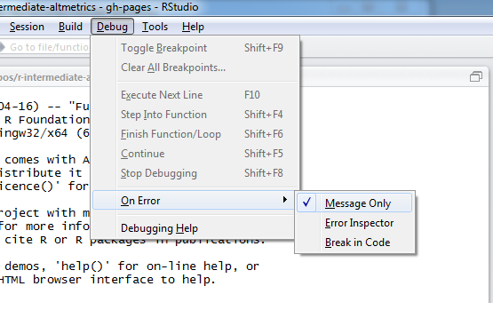
Configure RStudio debugging options

Recall the function we wrote earlier to calculate the mean of a metric for each level of a factor.

mean_metric_per_var <- function(metric, variable) {
  result <- numeric(length = length(levels(variable)))
  names(result) <- levels(variable)
  for (v in levels(variable)) {
    result[v] <- mean(metric[variable == v])
  }
  return(result)
}

And recall we invoke it as follows.

mean_metric_per_var(counts_raw$backtweetsCount, counts_raw$journal)

      pbio       pcbi       pgen       pmed       pntd       pone 
0.05557700 0.20624593 0.06387790 0.22574055 0.03133159 0.49421945 
      ppat 
0.03848541 

However, what can we do if we obtain an unexpected result? For example, let’s calculate the mean the number of tweets per year.

mean_metric_per_var(counts_raw$backtweetsCount, counts_raw$year)

numeric(0)

Strange. But how do we figure out what exactly is happening? Recall that the variables defined inside the function are not available outside in the global environment.

result

Error in eval(expr, envir, enclos): object 'result' not found

One option is to add print statements to the function to inform us the values of the variables in inside the function.

mean_metric_per_var <- function(metric, variable) {
  result <- numeric(length = length(levels(variable)))
  names(result) <- levels(variable)
  print(result)
  for (v in levels(variable)) {
    result[v] <- mean(metric[variable == v])
    print(result)
  }
  return(result)
}

And then re-run the function.

mean_metric_per_var(counts_raw$backtweetsCount, counts_raw$year)

numeric(0)

numeric(0)

While this strategy can often be effective, in this case it was not very informative. Also, we had to edit our function and all we got was a glimpse at what was happening while the function was running. Let’s remove the print statements, and re-define the function before trying a new strategy.

mean_metric_per_var <- function(metric, variable) {
  result <- numeric(length = length(levels(variable)))
  names(result) <- levels(variable)
  for (v in levels(variable)) {
    result[v] <- mean(metric[variable == v])
  }
  return(result)
}

We’ll use the R function debug. As an argument, we pass the function that we wish to debug.

debug(mean_metric_per_var)

Now everytime we run the function mean_metric_per_var, we will be entered into R’s interactive debugging environment.

mean_metric_per_var(counts_raw$backtweetsCount, counts_raw$year)

debugging in: mean_metric_per_var(counts_raw$backtweetsCount, counts_raw$year)
debug at #1: {
    result <- numeric(length = length(levels(variable)))
    names(result) <- levels(variable)
    for (v in levels(variable)) {
        result[v] <- mean(metric[variable == v])
    }
    return(result)
}

Browse[2]> 

In the console, we are now in the debugging environment. Furthermore, RStudio opens the “Source Viewer”, which conveniently shows us where in the function we are. Inside the function, we can run R commands to investigate what is happening, which is much more flexible than having to write multiple print statements. For example, let’s list the defined variables.

Browse[2]> ls()

[1] "metric"   "variable"

Since we are at the beginning of the function, the only variables defined are the two arguments that were passed to the function. To continue with the debugging, we need to learn the debugging commands, which we can see by running help.

Browse[2]> help

n          next
s          step into
f          finish
c or cont  continue
Q          quit
where      show stack
help       show help
<expr>     evaluate expression

The most useful command is n for “next” because we can use it to step through the function line by line.

Browse[2]> n

debug at #2: result <- numeric(length = length(levels(variable)))

The output tells us that the next line of code to be executed is #2. Typing n again will execute line #2 and similarly provide a preview of line #3.

Browse[2]> n

debug at #3: names(result) <- levels(variable)

Now that result has been defined. Let’s inspect it.

Browse[2]> result

numeric(0)

As we learned from our earlier print statement, result is a numeric vector of length 0. We expect its length to be the number of levels of variable.

Browse[2]> levels(variable)

NULL

The levels for variable are not defined. Let’s run str on variable to learn how R is storing it.

Browse[2]> str(variable)

int [1:24331] 2003 2003 2003 2003 2003 2003 2003 2003 2003 2003 ...

Now we have found the problem! Levels are only defined for a factor variable, but year was stored as an integer (or numeric) vector. When R imported the data, it saw only numbers in this column, and therefore did not anticipate our use of this column as a factor.

Now that we have identified the problem, we want to exit the debugger. One option would be to use f for “finish”, which will run the rest of the function and then exit. But since we know it won’t work anyways, let’s use Q for “quit”.

Browse[2]> Q

Now we’ll update the function so that if variable is not a factor, the function will convert it. To do this we use a conditional statement to check if variable is a factor with is.factor, and then if needed convert it with as.factor.

mean_metric_per_var <- function(metric, variable) {
  if (!is.factor(variable)) {
    variable <- as.factor(variable)
  }
  result <- numeric(length = length(levels(variable)))
  names(result) <- levels(variable)
  for (v in levels(variable)) {
    result[v] <- mean(metric[variable == v])
  }
  return(result)
}

Since we have re-defined the function, we will no longer be entered into the debugger when we run the function.

mean_metric_per_var(counts_raw$backtweetsCount, counts_raw$year)

       2003        2004        2005        2006        2007        2008 
0.000000000 0.009578544 0.054976303 0.016170763 0.040122277 0.047532408 
       2009        2010 
0.351047202 0.704338789 

And now the function works as expected.

mean_metric_per_var(counts_raw$backtweetsCount[counts_raw$journal %in% c("pbio", "pone")],
                   counts_raw$journal[counts_raw$journal %in% c("pbio", "pone")])

     pbio      pcbi      pgen      pmed      pntd      pone      ppat 
0.0555770       NaN       NaN       NaN       NaN 0.4942194       NaN